Book review

Summary

Turing wrote two very important papers for computer science: one in which he describes the Turing machine and the other in which he describes the Turing test for artificial intelligence.

Charles Petzold, of Windows books fame, had a pet project: explain the Turing machine paper. The original paper had about 30 pages and it’s a difficult read without context. In “The Annotated Turing”, at a ratio of about 30 pages of explanation to 1 of the original, Charles Petzold makes Turing’s paper readable by mere mortals.

Subject

Despite it’s importance for computer science, Turing’s paper is a mathematical one. The title is ‘On computable numbers, with an application to «insert long German word here»’

The long German word is one that was used in 1900 by David Hilbert at a mathematics conference. There David Hilbert presented 23 problems that mathematicians should work over the next century. The 10th problem referred to an ancient Greek mathematician: Diophantus.

Diophantus left a number of problems. One such problem sounds something like: “I stopped being a child at a sixth of my life, some other detail happened at a seventh, some years later I had a child, but he died when he was half my age; what’s my age?”. Being an ancient Greek the solutions must be integers or rational numbers; zero or irrational numbers a no-go areas. The issue is that there are no (or few) general approaches to solve his puzzles. In the example I gave, one would look for a number that is multiple of 6 and 7 and meets the other criteria.

So now back to David Hilbert, the challenge he proposes is: look, it’s unacceptable to not know. We need an algorithm that will decide if a Diophantine equation has or not a solution. He was not asking for an algorithm to solve, just to decide if a solution exists. The long German word that Turing refers to is decidability.

Turing describes the machine so that at the end he can say: and therefore there is no algorithm that can decide as per David Hilbert’s problem.

The machine

The machine is quite basic by today’s standards: it’s a state machine with a tape and a head to read and write symbols on the tape cells.

The state machine is a table with rows describing: given the current state and the current read symbol from tape at head what symbol to write on tape at head, how to change the head position (move left, right or no change) and what’s the next state. The tape has a beginning, but it’s unbounded at the other end.

A conventional usage of the machine is to generate a number. For this the tape has different usage for even and odd cells. It uses the even cells to print 0s or 1s, never skipping or re-writing with a different value such a cell, while the odd positions are used with a variety of other symbols for intermediate results. The 0s and 1s in the even cells are interpreted as a binary number between the integers 0 and 1.

E.g. if the machine prints 1 and then forever 0 this is interpreted as 0.10000…(binary) = 0.5(decimal). Here is for example such a machine:

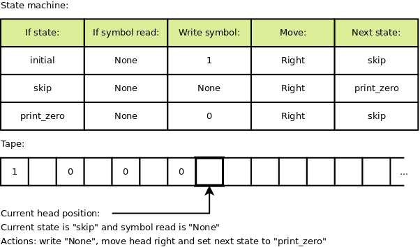
It’s not an efficient machine. The purpose of presenting the machine is to solve a mathematical question, not runtime efficiency.

The universal machine is a special program that interprets and execute the code of any other program. It turns out that all computers and languages that can emulate this universal machine (Turing complete) are equivalent (efficiency aside).

0s and 1s

We take it for granted that we’re using 0s and 1s in computers. But it’s not an obvious choice for 1936. The reason has to do with the state machine table. State machines tables for algorithms like incrementing a number are smaller when using binary:

• if 0 make it 1
• if 1 make it 0 and carry

Compare it with decimal:

• if 0 make it 1
• if 1 make it 2
• if 2 make it 3
• and so on
• if 8 make it 9
• if 9 make it 0 and carry

Functions

The other insight was that Turing introduced functions (i.e. procedures), without which the code for the state machine tables get big quickly.

The first function he introduces is a linear find, which he correctly identified as a fundamental algorithm. It’s behaviour is basically identical to the C++ STL linear find: if the value is found the head stops at the found value, otherwise the head stops on the tape at one past the last entry on tape.

There is no if syntax, so the find function receives, in addition to the value to find, two other functions: the function to call when a value is found, and the function to call when the value is not found. The idea of functions as arguments is again ahead of it’s age.

And the last item is that shortly after introducing functions, he uses overloads i.e. same function name, but with a different number of parameters. For example the C language, introduced in early 1970s did not have overloads, they were added later to C++.

Enumerating

A lot of the following comes from Cantor; it’s still fun.

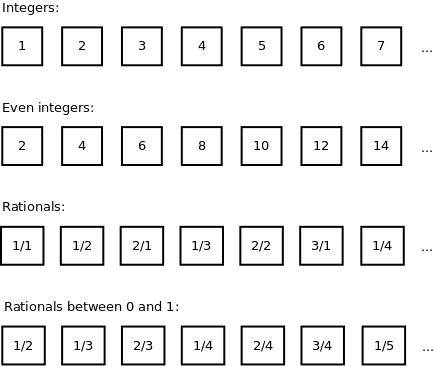
So, we can enumerate/count integers: 1, 2, 3, 4, 5, 6, 7, and so on.

So if we have a proper subset such as the even integers: are there more or less then the set of all integers. On one side there a less, more specifically the set of even integers does not include any odd integer. But on the other side we can still do a one to one mapping between each integer and the even integers: 1 <-> 2, 2 <-> 3, 3 <-> 6, 4 <-> 8, 5 <-> 10, 6 <-> 12, 7 <-> 14 and so on. Therefore there are about the same even integers as integers.

How about rational numbers, expressed as a ratio of two integers? Well, they are about as many as the integers. We can order them by the sum of the two integers in the ration: (sum 2) 1/1, (sum 3) 1/2, 2/1, (sum 4) 1/3, 2/2, 3/1, (sum 5) 1/4, and so on. Therefore there are about as many rational numbers as there are integers.

And there are about as many rational numbers between 0 and 1 as there are rational numbers greater than 1. We can define a function f(x) = 1 / x that puts the two sets into correspondence. E.g. 2/5 corresponds to 5/2 in the other set. This is counter-intuitive because as rational numbers greater than 1 include an infinity of intervals as big as between 0 and 1: e.g. the ones between 1 and 2, the ones between 2 and 3, and so on.

Reals

Now as far as the real numbers, that could have an infinite number of decimals, we’re talking of a lot more. But not all real numbers are the same.

For example square root of 2 is not rational. This has a sweet little reductio ad absurdum proof. But square root of 2 is a solution of an algebraic equation. And algebraic equations can be ordered by a trick similar to the one we used for rational numbers. Therefore square root of 2 is part of a enumerable set, the solutions for algebraic equations, set that also includes all the rational numbers.

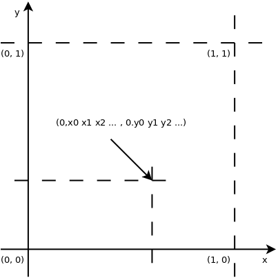
Also there are about as many real numbers between 0 and 1 as there are real numbers greater than 1. Also in the square in a plane with x between 0 and 1, y between 0 and 1 there are only as many as on a line between 0 and 1. That’s because the coordinate of the dot in the square look like 0.x0 x1 x2 ... and 0.y0 y1 y2 ... (where xi and yi are digits) and they have a 1 to 1 correspondence to the number 0.x0 y0 x1 y1 x2 y2 .... And in general there are as many real dots in a N dimensional cube as there are reals between 0 and 1.

This hopefully explains why Turing’s focus on algorithms generating numbers between 0 and 1.

Computable numbers

So what numbers can we generate with an algorithm? We can generate integers, rationals, but how about real numbers? We can generate square root of 2, π (3.14159…), but counter-intuitively we can’t generate all the reals. That’s because there are more reals than integers. Reals can’t be enumerated.

Algorithms on the other side can be compiled to a executable, then we can order the binaries. We can order them by the size of the executable file and, within the executables of the same size, by the actual number of the binary of the executable (i.e. the processor instructions). Therefore the cardinality of the algorithms is smaller than the one for real numbers. Therefore we can’t calculate all the reals with algorithms.

Correctness

One important intermediate result from the Turing paper is the impossibility to create a generic algorithm to verify correctness of a program.

The demonstration uses reductio ad absurdum.

Suppose we care about algorithms that have the conventional behaviour mentioned above of printing a binary number between 0 and 1. Let’s call such algorithm satisfactory.

Let’s assume there is an algorithm D that can decide if binary program corresponds to a satisfactory algorithm. E.g. it would first check first things like valid instructions, cases where 0s or 1s are erased, cases where the machine loops forever without making progress etc. and return false. For satisfactory algorithms it would return true.

Then let’s build another machine H. This machine put together:

• a couple of counters starting at 0
• the decision algorithm D
• and the universal machine UM

Machine H in a loop:

• increments counter C
• interprets the value of C as an algorithm
• pass C as input to D
• if D return true
  • increment counter N
  • pass C as input to UM, run until it generate it’s Nth digit
  • print that digit

It’s all potentially good until C contains the binary of the machine H.

Then if D returns false, H cannot be build. If D return true, this results in infinite recursion.

Therefore the assumption that D exists is false.

Implications

Here are some implications.

There is no general algorithm to determine the correctness of an arbitrary program.

However there is hope. Algorithms can be designed to be correct.

For code reviews it means that requests towards the reviewer to “Find what’s wrong with this code” are impossible. The right approach is for to provide reason upfront “Here is why this code is correct”.

This also explains why neural network algorithms tend to have false positives. It’s because by adjusting weights to minimise the error, they find some algorithm. There is no guarantee that the algorithm is correct (and no general way to determine correctness).

Other

As an interesting fact Charles Petzold tells a story of the origin of the lambdas (as in Lisp/Scheme lambdas). The usage was introduced by Alonzo Church, for lambda calculus, a mathematical approach equivalent to the Turing machines. A previous notation used by Whitehead and Russell used a caret ^ character on top of x. Church wanted to put the caret in from of the character as in ^x, but for printing related reasons the caret became λ instead.